SAE Training — Building the Prism

The Training panel is where you build the Sparse Autoencoder that decomposes polysemantic neurons into monosemantic features.

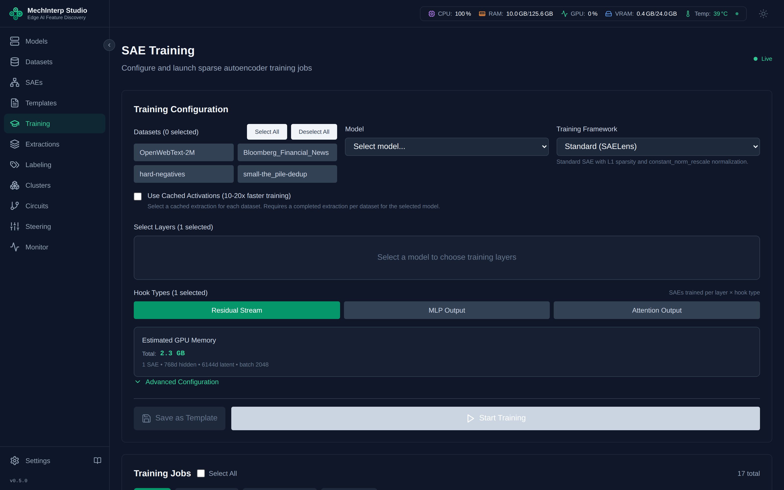
Configuring a Training Job

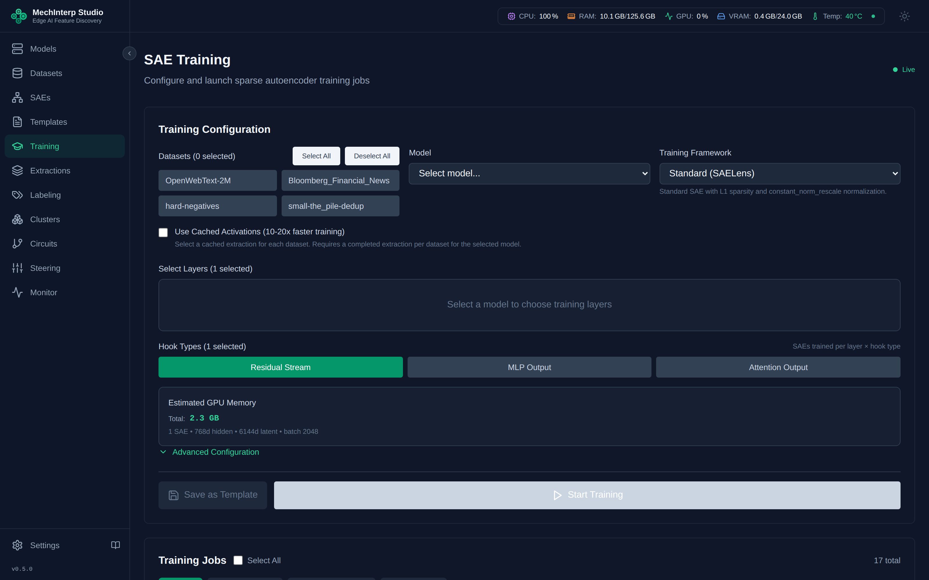
The training configuration walks you through three steps: select a model, choose your SAE architecture, and set hyperparameters.

The Six SAE Frameworks

miStudio supports six paper-grounded SAE architectures, each with different sparsity mechanisms and trade-offs:

1. Standard SAELens (Bricken et al., 2023)

The classic approach — ReLU activation with L1 sparsity penalty.

Parameter	Default	Description
l1_alpha	5e-4	L1 penalty strength. Higher = sparser but risks dead features
normalize_activations	constant_norm_rescale	Rescales activations to unit norm before encoding

When to use: General-purpose feature discovery. Good starting point for new researchers.

L1 Tuning Guide

• Too many messy features? Increase l1_alpha (try 2x)
• Too many dead features (>50%)? Decrease l1_alpha (try 0.5x)
• Target: L0 between 10–100 active features per token, dead neurons <20%

2. Standard Anthropic (Templeton et al., 2024)

Anthropic's variant with specialized normalization and higher default sparsity.

Parameter	Default	Description
l1_alpha	5.0	Much higher than SAELens — Anthropic's normalization rescales differently
normalize_activations	anthropic_rescale	Anthropic-specific rescaling that changes the L1 coefficient scale

L1 Scale Warning

The l1_alpha for Anthropic (default 5.0) is NOT comparable to SAELens (default 5e-4). The normalization modes change what the coefficient means. Do NOT copy L1 values between frameworks.

When to use: When replicating Anthropic's published results or using their recommended configurations.

3. JumpReLU (Rajamanoharan et al., 2024 — Gemma Scope)

High-performance architecture using learnable thresholds. Features are binary — OFF below threshold, full activation above.

Parameter	Default	Range	Description
sparsity_coeff (λ)	1e-3	1e-5 to 5e-3	L0 coefficient (paper scale). At L0=50: loss_l0 = 1e-3 × 50 = 0.05
initial_threshold	0.5	0–5.0	Starting jump threshold per feature
bandwidth	0.01	0–1.0	STE gradient estimation bandwidth
normalize_decoder	true	—	Required: keeps decoder columns at unit norm

How it works: Instead of a continuous penalty, JumpReLU uses a step function approximated by a sigmoid for gradient flow: σ((z-θ)/ε) where θ is a learnable per-feature threshold. Features are counted (not averaged) for the L0 loss: L0 = Σ_i H(z_i - θ_i) summed per sample, then averaged over the batch.

Sparsity Coefficient Scale

sparsity_coeff for JumpReLU is on a completely different scale than l1_alpha. Typical values: 1e-4 to 5e-3. Do NOT use L1 values (like 0.0005) for this parameter — they will produce zero sparsity pressure.

When to use: Best for preventing "shrinkage" — features activate sharply rather than being penalized into small values. Preferred for production-quality SAEs.

4. TopK (Gao et al., 2024 — OpenAI)

Structural sparsity — exactly K features activate per input, no penalty needed.

Parameter	Default	Description
top_k	64	Exact number of active features per sample
aux_loss_alpha	0.03125	Auxiliary loss weight for dead feature prevention (1/32 per paper)
aux_k	top_k × 2	Features used in auxiliary loss computation
adam_epsilon	6.25e-10	Paper-specific Adam optimizer epsilon

How it works: After encoding, only the top K activations are kept; all others are zeroed. An auxiliary loss encourages dead features to eventually activate.

When to use: When you want exact control over sparsity level. No L1/L0 tuning needed — just set K.

5. Skip (Community Variant)

Standard L1 sparsity with a residual skip connection from input to decoder output.

When to use: When reconstruction quality is critical — the skip connection provides an "escape hatch" for information the SAE bottleneck can't capture.

6. Transcoder (Dunefsky et al., 2024)

Predicts MLP output from MLP input — learns the transformation a layer performs.

When to use: When studying how information transforms between layers, not just what's represented at a single point.

Framework-Aware Configuration

When you select a framework, the UI automatically:

• Shows/hides framework-specific fields (e.g., top_k only appears for TopK)
• Sets paper-grounded defaults for all parameters
• Adjusts validation ranges to match the framework's expected scales

Activation Normalization Modes

Before feeding activations into the SAE, they can be normalized:

Mode	Description	Used By
constant_norm_rescale	Rescale to constant L2 norm	SAELens Standard
anthropic_rescale	Anthropic-specific rescaling	Standard Anthropic
none	Raw activations, no normalization	Skip, Transcoder

Why Normalization Matters

Different normalization modes change the scale of activations entering the encoder, which changes the effective meaning of sparsity coefficients. This is why l1_alpha=5.0 for Anthropic produces similar sparsity to l1_alpha=0.0005 for SAELens — the normalization absorbs the difference.

Essential Hyperparameters

Beyond architecture-specific settings, these apply to all frameworks:

Parameter	Default	Range	Effect
Learning Rate	framework-dependent	1e-5 to 1e-2	If loss spikes: too high. If loss barely moves: too low.
Batch Size	4096	32–65536	Larger = smoother gradients but more VRAM
Total Steps	30,000	1,000–1,000,000	More steps = better features, longer training
Warmup Steps	1,000	0–10,000	Linear LR warmup prevents early instability
LR Decay Steps	0 (off)	0–total steps	Linear decay of the learning rate to 0 over the final N steps. Warmup + decay must not exceed total steps.
Sparsity Warmup	5,000	0–50,000	Gradually increases sparsity pressure. Critical for JumpReLU to prevent mass neuron death at initialization.
Expansion Factor	8–32×	2–128×	SAE width relative to model hidden dim. 8× is common (512 neurons → 4,096 features).
Weight Decay	0.0	0–0.1	L2 regularization. Usually 0 for SAEs.
Gradient Clip Norm	1.0	0–10.0	Prevents gradient explosions during training.

Learning rate is per-framework

Selecting a framework sets its paper-grounded learning rate automatically. The defaults are 4e-4 for Standard SAELens, Standard Anthropic, Skip, and Transcoder; 3e-4 for TopK; and 7e-5 for JumpReLU. Override the value only if you have a reason to — the defaults track each paper's recommended setup.

Dead Neuron Management

Features that never activate are "dead neurons" — wasted capacity.

Setting	Default	Description
dead_neuron_threshold	1,000 steps (the form suggests 10,000)	A feature is dead once it has not fired on a single token for this many consecutive training steps
resample_dead_neurons	true	Re-initialise dead features at each resample
resample_interval	5,000 steps	How often to resample: only after both warmups, and never inside the LR decay window

Every framework except TopK resamples, JumpReLU included. A resample follows the Anthropic recipe, in the normalised space the encoder actually sees:

• inputs from the current batch are picked with probability proportional to the square of their reconstruction loss;
• the dead feature's encoder row points along that input (centred), at a fifth of the average encoder norm of the features still alive, and its decoder column is the same direction at unit length;
• its encoder bias is zeroed, and for JumpReLU its threshold is set to half the feature's activation on that input, so it fires on it;
• the optimizer's moments for exactly those weights are reset.

The dead-neuron count in the training metrics is a separate, faster-moving activity estimate, so it can differ from the number a resample reports.

Dead Neuron Debugging

• >50% dead: Your sparsity pressure is too high. Reduce l1_alpha or sparsity_coeff.
• <5% dead: Your sparsity might be too low — features may be polysemantic.
• 10–20% dead is typical and healthy.
• TopK: Uses auxiliary loss instead of resampling — set aux_loss_alpha higher if too many die.

Training Metrics

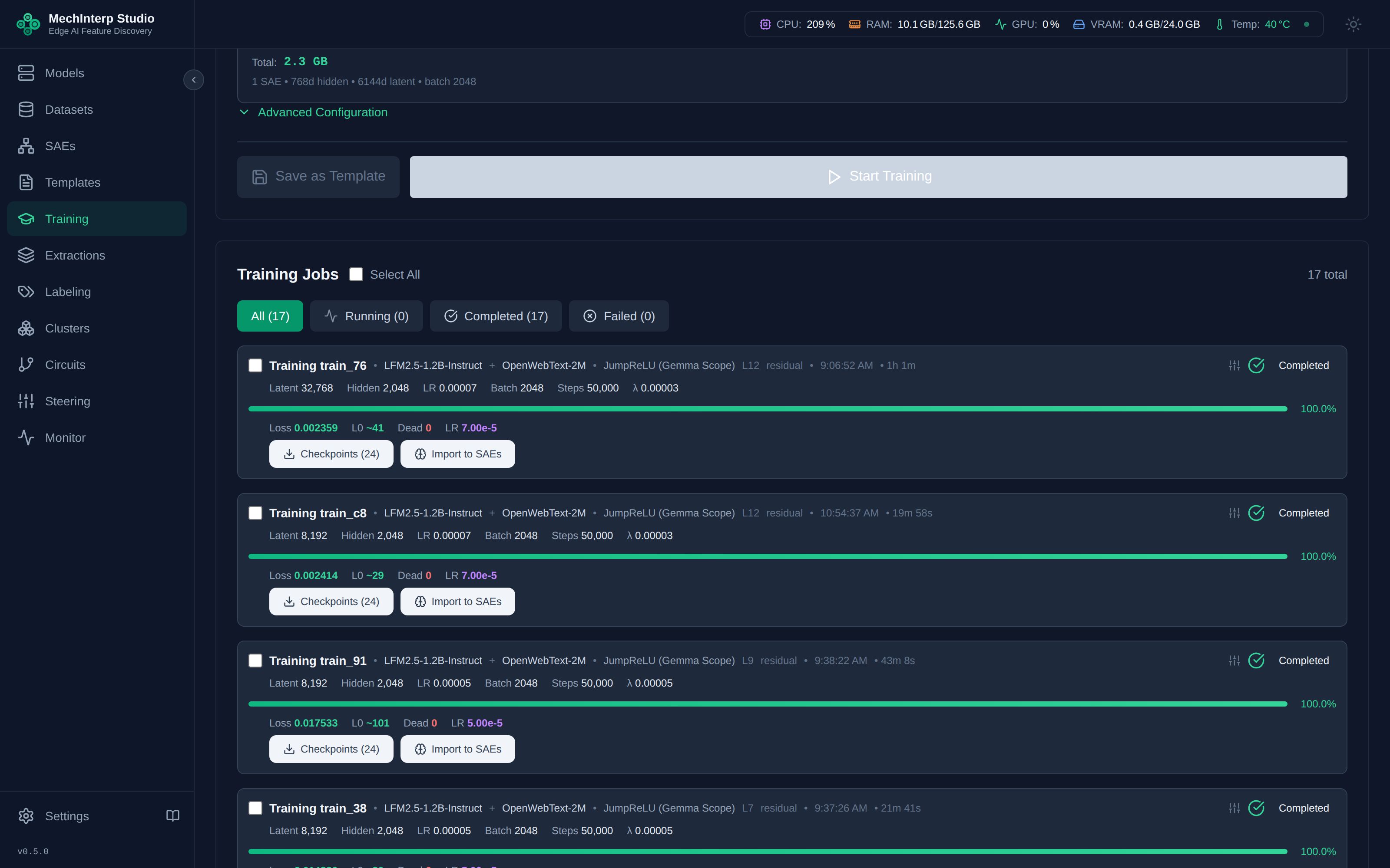
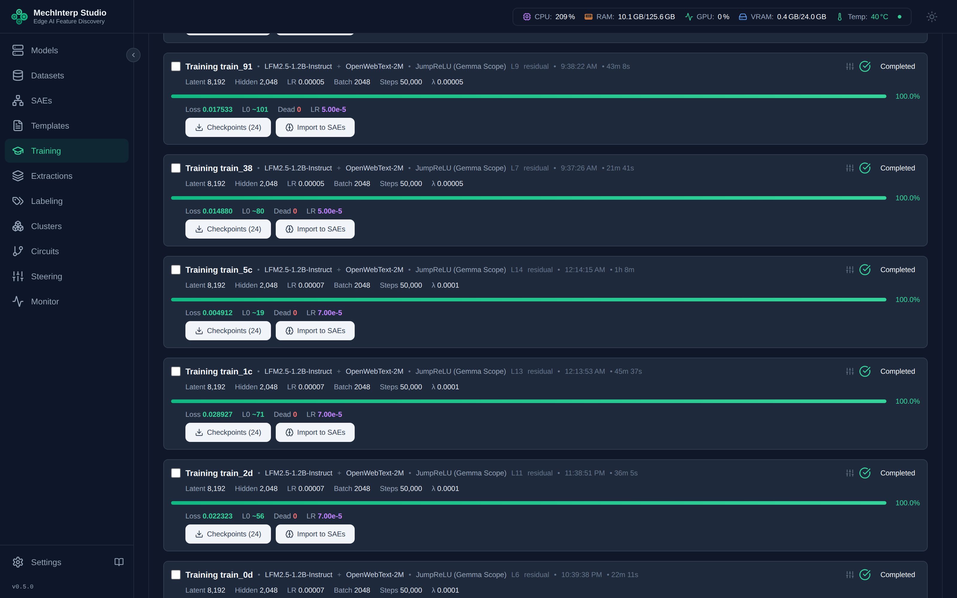
While training, miStudio streams these metrics in real-time via WebSocket:

Metric	Target	What It Means
Total Loss	Decreasing	Combined reconstruction + sparsity loss
Reconstruction Loss (MSE)	< 0.1	How much "truth" the SAE lost. Lower = more faithful.
L0 (Sparsity)	10–100	Average active features per token. Lower = easier to interpret.
FVU	See below	Fraction of Variance Unexplained: the share of the activations' variance the reconstruction misses. 0 is perfect; 1 is no better than predicting the mean.
Dead Neurons %	10–20%	Features that never fire. See Dead Neuron Management above.

Reading the training card

The card is the live view of a run, and a few of its conventions are worth knowing:

• L0 is shown as a count, not a fraction. The card, its log lines and Copy logs all report L0 as the number of active features with the percentage beside it — L0: 7 (0.02%), not L0: 0.000. The 10–100 target above is in those units. On a wide dictionary the fraction rounds to zero long before the count does.
• The L0 chart carries a first → latest trend, also in counts, so a slow drift is readable without reading off individual points.
• The window is the last 1,000 logged steps, which covers a full-length run rather than a recent sliver.
• A missing point is drawn as a gap, never as zero — a gap in reporting is not a run that reached zero sparsity.
• A completion ETA appears in your own timezone, computed from the recent step rate. It is deliberately absent for runs that are finished, paused, or have not reported in a while, because an estimate from a stalled clock recedes rather than converging.

Reading FVU

miStudio reports FVU as Σ‖x − x̂‖² / Σ‖x − μ‖², where μ is the mean of each activation dimension. This is the standard definition, and every SAE framework reports it.

There is no universal good value. FVU depends on the model, the layer, the corpus and the sparsity, so compare runs at a similar L0 rather than against a fixed number. As a reference, train_6247e768 (LFM2.5-1.2B, residual stream at layers 11–13, JumpReLU with 8,192 latents, about 65 active per token) measured 0.26–0.32 on held-out text. That run reconstructs most of the variance and still costs the model about 0.3 nats of cross-entropy per spliced layer. FVU alone did not show that; the model-cost evaluation does.

Compare FVU within a layer, never across layers

FVU measures reconstruction error in each layer's own activation space, and the same error costs the model different amounts depending on where in the stack it sits. So a lower FVU does not mean a better SAE when the two layers differ.

Measured on one 16,384-feature run training three adjacent layers together:

Layer	FVU (held-out)	Loss recovered vs mean-ablated
11	0.2445 — best	94.49%
12	0.2967	95.37% — best
13	0.2967	94.26%

FVU ranks layer 11 first by a clear margin. What the SAE actually costs the model ranks layer 12 first, with all three within about one point of each other. To compare SAEs across layers, use loss recovered vs mean-ablated from the model-cost evaluation. Use FVU to compare runs at the same layer.

Older runs show a legacy FVU, and it reads lower

Runs recorded before 2026-09-15 stored a different formula: var(x − x̂) / var(x) with one mean over every element. On activations with large, nearly constant dimensions that value reads low: 0.26 where the standard formula gives 0.32 at LFM2.5-1.2B layer 11. The card labels such a value FVU (legacy) and never shows it as plain FVU. New runs record both; the legacy value appears beside the headline only for comparison with older runs. The guidance this page used to give ("below 0.1, below 0.05 excellent") was calibrated to the legacy formula, and it does not apply to FVU as reported now.

Model-Cost Evaluation

Every metric above lives in the SAE's own space. None of them says what the reconstruction costs the model. When a training completes, miStudio splices each residual-stream SAE back into the base model and measures next-token cross-entropy on text the training never read. The results appear in the Model-cost evaluation panel on the training card.

Column	Meaning
CE spliced (Δ)	Cross-entropy with the SAE's reconstruction in place of the layer output, and its change from the untouched model.
Recovered vs mean	(mean-ablated − spliced) / (mean-ablated − base), where the mean-ablated run replaces the layer output with its mean activation. 100% means the SAE costs the model nothing; 0% means it is no better than that mean. This is the headline.
vs zero	The same ratio against zeroing the layer. Zeroing a residual layer makes these models emit a near-uniform distribution, so almost any SAE scores near 100% here. It is shown for reference only.
KL	KL divergence from the untouched model's next-token distribution, in nats per token.
L0 / FVU	Measured on the same unseen text.
All	Cross-entropy with every layer's SAE spliced in at once.

Which text. An extraction reads the first max_samples rows of its tokenization, so rows at or above that bound were never seen by an SAE trained on it. The evaluation reads only those rows, split across sources in proportion to the training mixture. When a training reads two extractions of the same tokenization, the larger bound applies to both, so a row either extraction read is never evaluated. The budget is evaluation_token_budget (default 131,072 tokens). A training that extracts activations on the fly reads its rows from the whole tokenization, so only the rows it held out (holdout_fraction above 0) are guaranteed unseen: its evaluation reads those, and is recorded as skipped, with the reason, when nothing was held out.

"Unseen" and "comparable" are not the same claim

Because both the training prefix and the held-out remainder are positional, what the evaluation measures depends on the block order of the tokenization — check shuffled on it before comparing numbers across runs.

• Shuffled (the default when a tokenization is written): the prefix is a uniform sample of the corpus and the held-out rows are drawn from the same distribution. The evaluation then measures generalisation, which is what these numbers are for.
• Corpus order (shuffled not set): the prefix is the corpus's opening slice and the held-out rows are its tail. Those can be materially different text — OpenHermes-2.5, for instance, is written one source at a time, so its first 10% of rows holds 2 of its 15 sources. The held-out rows are still genuinely unseen, but a score against them reflects a distribution shift as much as it reflects the SAE.

The same applies to the mixture: each corpus contributes its own tokenization's block order independently, so a mixture can be uniform in some sources and positional in others.

Evaluating an older training. Press Evaluate on a completed training's card, or call POST /api/v1/trainings/{id}/evaluate. This runs as a GPU job: it loads the base model and the exported SAEs, and the result appears on the card when it finishes. A failure is recorded with its reason and never changes the training's status. Only residual-stream SAEs can be spliced; a transcoder or an attention or MLP SAE is listed as skipped, with the reason.

If an evaluation stops. A running evaluation rewrites its record about once a minute. If its worker is killed (a pod restart, an out-of-memory kill), the stuck-job janitor marks it failed once its record is ten minutes old and its task is no longer running. A request that stays pending is never failed automatically, because it may be queued behind a long job; after 15 minutes without an update the panel offers Force re-run.

Set evaluate_ce_delta: false to skip the evaluation after training.

Held-out rows during training. With holdout_fraction above 0, every log step also scores held-out text the SAE never trains on: holdout_eval_tokens per layer (default 100,000), drawn across sources in proportion to dataset_weights (in equal shares when there are none), in forward passes of holdout_eval_chunk_tokens (default 2,048). The chunk size changes memory, about 16 bytes × latents + 64 bytes × width per token, never the result.

Training Controls

Active training jobs support:

• Pause / Resume: Suspend training to free the GPU for other work, then continue after the newest complete checkpoint. The optimizer, learning-rate schedule, dead-latent statistics, random number generators and data position are restored, so the run continues as if it had never stopped. A pause writes its own checkpoint at the step it stops (one step later when it arrives just after an out-of-memory retry), so no step is repeated; after a crash the run resumes from the newest periodic checkpoint and repeats the steps after it. If the resumed process cannot hold the activation buffer the run started with (it has less free memory), the buffer is re-planned. The run still never repeats a token or trains on a held-out row, but it no longer continues bit-identically, except when a whole activation pool only moved between the GPU and host memory, which continues exactly. The checkpoint records the outcome in resume_history.
• Stop: End the run. Its checkpoints remain on disk, but no importable SAE is produced.
• Stop & Finalize: End the run and build the SAE from the newest checkpoint, so it stays importable.
• After training finishes: a run is marked Completed as soon as its full-length export is saved, before the post-run evaluation. During that evaluation Stop and Stop & Finalize cancel only the evaluation, Pause is refused, and Finalize is refused because it would replace the final weights. The card shows no Stop button then; use POST /api/v1/trainings/{id}/control with {"action": "stop"}.
• Checkpoints: Saved every N steps (configurable). Each records loss, L0 and model weights, plus training_state.pt with everything a resume restores, so a checkpoint step takes about three times the weights on disk (16K latents over three LFM2.5-1.2B layers: about 2.4 GB per step). A checkpoint that falls inside a gradient-accumulation window also saves the gradients, which adds the weights' size again. Nothing checks free disk space before a save, and a save that fills the disk fails the run. Budget the disk for every checkpoint the run will write, because retention never prunes an active run. Choose the interval with that in mind. The best checkpoint (lowest loss) is tracked automatically. A multi-layer run saves one checkpoint per layer per step.

Stop does not save an importable SAE

Stopping a run leaves its checkpoints in place but does not write the Community Standard export that every downstream feature reads — so the model will not appear under Import to SAEs. Use Stop & Finalize, or click Finalize on the stopped run afterwards.

See Training Lifecycle & Checkpoints.

Training Templates

Save any training configuration as a template for reproducibility:

• Export as JSON to share with colleagues
• Import templates from other researchers
• Mark favorites for quick access
• Duplicate and modify for parameter sweeps