Probe Monitors — A Detector, and Honest Evidence About It
A probe monitor is a small linear readout over one decoder layer's residual stream: a vector and a threshold that answer is this concept present in what the model is processing right now? Nothing about it is exotic — it is logistic regression on activations. What the panel is really for is the second half: finding out how well it actually works, and not overstating it.
A probe is cheap to run next to a model, which is the whole appeal. A 7B judge reading the same text costs a forward pass per check; a probe costs a dot product. That trade is only worth making if you know what you are giving up, so this feature spends most of its effort on measurement.
What a probe is, exactly
It helps to be concrete, because the word "probe" invites a mental model that fits only half of what miStudio builds.
The dense probe: one vector, no latents
A dense probe — the default, and what the tile labels dense residual — is literally this:
weight   d_model numbers   (2,048 for LFM2.5-1.2B, 4,096 for Llama-3.1-8B)
bias     1 number

score(token) = standardise(activation at layer L) · weight + bias
That is the entire artifact. There are no feature detectors inside it, nothing that "activates", and no dictionary. It is one dot product against the residual stream, which is why it costs almost nothing to run beside a model: the forward pass was happening anyway, and the probe adds a vector multiply at one layer.
The k-sparse SAE probe: one weight per latent
A probe can instead read an SAE's feature basis. Training encodes the activations through the SAE, ranks the features by a standardised class-mean difference on the training rows only, keeps the top k, and learns one weight per kept feature.
This is the version where "latents activate and the probe reads them" is an accurate description.
The tile shows it as an SAE basis with its feature count instead of dense residual.
| dense | k-sparse SAE | |
|---|---|---|
| what it reads | the raw residual stream | the SAE's feature activations |
| size | d_model weights | k weights |
| needs an SAE? | no | yes, and a published one to export |
| interpretable per-weight? | not really | yes — each weight names a feature |
It is never told which tokens matter
Worth knowing before you read a token trace: training minimises binary cross-entropy on the pooled aggregate against the whole-input label. Nothing supervises individual tokens. The per-token scores the trace shows are a by-product you can inspect, not a target the probe was fitted to. That is why a single strongly-coloured token does not mean "the probe fired here".
The evidence ladder
Every probe carries a rung, and the rung is computed from the evidence, never asserted:
| rung | what it means |
|---|---|
| 0 | trained — a probe exists and fit its training data |
| 1 | detects on held-out data — it works on rows it did not see, from the same distribution |
| 2 | detects on unseen tasks — it works on an out-of-distribution evaluation set, with the lower bound of a bootstrapped confidence interval clearing chance |
| 3 | detects on unseen tasks, compared with a judge — an LLM judge scored the same rows, so the probe's number has something to be read against |
Two things about rung 3 are deliberate and easy to misread.
"Compared with", not "beats". A probe at rung 3 has been measured against a judge. It may have lost. On the reference run it did lose — the judge averaged 0.8744 across five sets against the probe's 0.7938, and won on all five individually. That is recorded rather than buried, because a rung-3 badge could otherwise be read as "better than asking a model", which it does not mean. The probe's case on a small model is cost and latency, not accuracy.
The rung moves, and a stale export is invalidated. Run another evaluation or a judge pass and the rung is recomputed. If it changes, any definition already built is marked invalidated rather than silently left in place — a cached document stating an old rung is a lie that still parses.
Running one, field by field
The panel is Probes in the sidebar, between Circuits and J-Lens. Everything needed to start a run is on that one page, above the list of past runs. Filling it in, top to bottom:
| control | what to put in it |
|---|---|
| Model | The model whose residual stream you are reading. It must already be downloaded (Models panel). |
| Training view | The labelled dataset the probe learns from. This is a view, not a raw dataset — see below. |
| Evaluation sets | Tick any number. Each is marked OOD (out-of-distribution) or in-distribution, and that marking is what decides whether a run can reach rung 2. |
| Calibration set | Leave as "none — use validation negatives" unless you have a set of known-negatives you would rather calibrate the threshold on. |
| Scope | all, assistant, user or last_assistant. The panel says it plainly: these are different detectors, not a preference. |
| GPU | Auto — most free memory is right almost always. |
| Layers | stride walks the stack (stride 5 over 16 layers gives layers 1, 6, 11); explicit takes a list like 11,12,13. The run trains a probe at each and keeps the best. |
| Rules | The pooling rules to try: mean, max, last, softmax, attention, rolling_mean_max. Tick several — the run picks the winner by validation AUROC and shows you the whole sweep. |
| Max length | Token cap per row. 4096 is the default. |
| Top-N layers | How many layers to carry forward from the sweep. 1 is normal. |
| Target FPR | The false-positive rate the threshold is calibrated to. 0.01 is the default. |
| Seed | 1337 by default. The same seed gives the same split, the same capture order and the same initialisation — which is what makes two runs comparable. |
| SAE variant | Also trains a k-sparse probe over an SAE basis. It needs a ready residual SAE for that model at the selected layer, or the run is refused naming the layer. |
Then Start probe run.
If "Training view" is empty, that is the step you are missing
A probe cannot read a raw dataset. It needs a view: which column holds the text, which column
holds the label, and what each raw label value means — positive, negative or excluded. A view
that cannot produce both classes is refused when you create it, rather than forty minutes into a run.
Views are created against a dataset you have already downloaded, and each one is tagged with a
role (train, eval or calibration) and, for evaluation views, a distribution
(in-distribution or OOD). The existing views on this installation are named like
models-under-pressure training (train) and models-under-pressure mt_balanced — one training view
and five OOD evaluation sets over the same source dataset.
What a good first run looks like
Nothing exotic: one model, the training view, all the evaluation sets, scope all, stride layers,
and two or three rules. That gives you a layer sweep to look at and a probe at the end. A run with
no evaluation sets is also allowed and gives you a rung-0 probe — worth doing if all you want to
know is whether a concept is linearly present at all.
Three settings that change the answer, not just the speed
Most of the form is bookkeeping. These three are not.
- Pooling rule. How per-token scores become one score for a row. On the reference corpus
meanreached 0.8841 out of distribution whileattentionreached 0.6986 — and the attention probe was not under-trained: it converged to a lower training loss and generalised far worse. Tick several and let the run choose. - Scope. Which tokens may be scored. Template scaffolding is never scored under any scope,
because including a BOS token would make a
meanrule's denominator depend on the chat template rather than on the text. - Layers. The run keeps the best by validation AUROC, and the tile says when that choice was close: "margin over the runner-up 0.0012 — a near-tie, so the chosen layer is close to arbitrary." Treat a near-tie as "any of these layers", not as a finding about layer 11.
What a run actually does
One run is not one probe. A run sweeps, trains, calibrates and evaluates, and hands back several probes for you to choose between. Its eight stages appear on the tile as it works, and a failure names the stage it failed at.
| stage | what happens |
|---|---|
rendering | each labelled row becomes the token ids the model will really see, with the chat template applied |
pooled_capture | the model runs over the training rows; one pooled activation is kept per row, per candidate layer |
layer_selection | the sweep — a cheap probe is fitted at every layer × pooling rule and scored on validation |
token_capture | the chosen layer is re-run, this time keeping per-token activations |
training | AdamW and BCE on the aggregate, early stopping on validation AUROC |
calibrating | the threshold is placed at the score that spends your target false-positive rate on validation negatives |
evaluating | the held-out sets are scored: AUROC, bootstrap CI, operating points |
rung | the evidence rung is derived from what actually ran |
Two details in there are easy to miss and change how you read the output.
Early stopping watches AUROC, not loss. They do not share a minimum. Stopping on loss can hand back a probe that separates the classes worse than one seen several epochs earlier.
The threshold is calibrated on validation negatives, and it rarely lands on your target. Asking for 1% typically yields something like 0.97% or 0.82%, because scores are discrete at the sample level. The tile shows what was actually spent, not what you asked for — those are different numbers and only one of them is true.
Why one run produces four tiles
mean, max, last and attention are four pooling rules over the same readout. The run scores
all four and selects a winner on validation AUROC, but keeps them all, because the winner
in-distribution is not always the winner out of it. On the reference run, attention reached a
lower training loss than mean and generalised distinctly worse — which is what overfitting
looks like when you have the evidence to see it.
Reading the run tiles
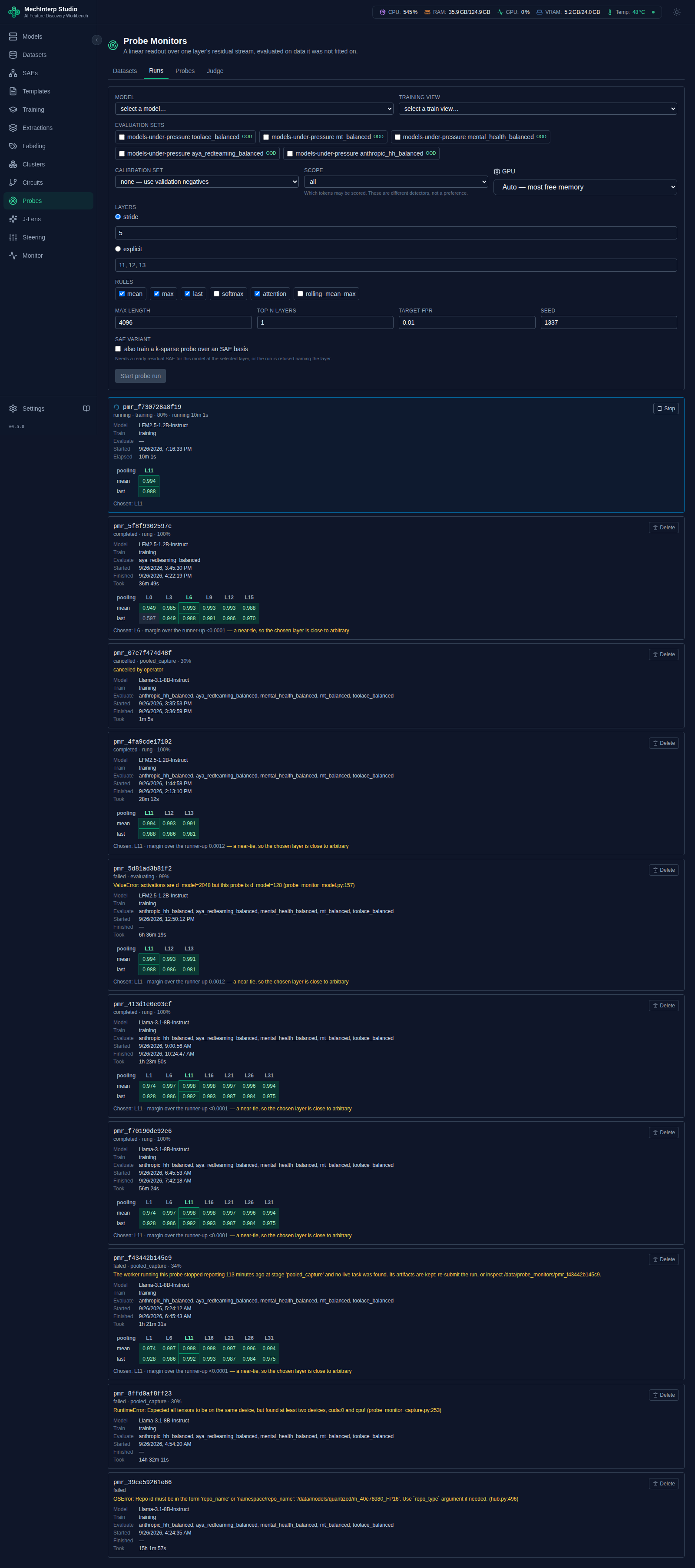
One tile per run, newest first. Each carries:
- the run id, its status, the stage it is in and a percentage — the stage matters, because
"40%" means nothing without
pooled_captureorevaluatingbeside it; - a spinner and a progress bar while it is live, the same bar every other running job in miStudio draws;
- the datasets it is actually using — model, training view, and every evaluation set by name rather than by id;
- when it started, when it finished, and how long it took;
- the layer sweep it chose from, as a small table of rule against layer, and which layer won.
A run that failed shows its error on the tile. A run whose end was never recorded shows
Took — rather than a duration counted up to the present moment: a made-up number is worse than a
blank, because you cannot tell it is made up.
Stop appears while a run is live and Delete once it is not. Stopping is cooperative — work halts at the next clean boundary rather than being killed, so the GPU is released properly and the row does not end up in a state nothing can read. Deleting removes the run, every probe trained in it, and its artifact directory, which is gigabytes of token capture; the tile asks first and says so.
Try it on your own text, and read the trace
Try it on your own text scores one input and shows what every token contributed. It is the fastest way to find out whether a probe reads the concept or reads something correlated with it.
The two colours
| meaning | |
|---|---|
| violet | this token pushed the score up — toward the concept |
| emerald | this token pushed the score down — away from it |
<|…|> chip | chat-template scaffolding, not your words |
| dotted underline | outside this probe's scope, so not scored at all |
That last row matters more than it looks. A token outside the scope has no score — it is not a zero. Shading it as "cold" would say the probe looked and found nothing, when it never looked.
Scaffolding is marked rather than hidden, deliberately. A probe firing on <|im_start|> rather
than on your sentence is a finding, and filtering those tokens out would delete the evidence for
it. With scope all, a chat-rendered input genuinely does score its template tokens.
The four bands, and what they are not
Shading is banded — faint, weak, moderate, strong — and each band moves three things together: background strength, text colour, and an underline rule. One channel alone is not legible across a long passage.
⚠ The bands rank tokens against each other within one input. They are cut against the 90th percentile of the magnitudes in that input, not against any fixed scale. Two consequences:
- Bands do not compare between two inputs. A "strong" token in a passage that scored far below threshold is still part of a low score.
- Two tokens in the same band are not ranked against each other. Hover for the exact number.
The percentile is there because the alternative does not work. Scores are heavy-tailed: on a real 90-token input the largest magnitude was 33.24 while the median was 4.23, so cutting bands against the maximum put 86 of those 90 tokens into the bottom two bands and the whole passage rendered as one flat wash.
Only the aggregate decides
The per-token scores are pooled by the probe's rule into a single aggregate, and the aggregate alone is compared with the threshold. A strongly-coloured token does not mean the probe fired, and a probe that fired does not mean any particular token caused it. The trace tells you where the signal was distributed; the aggregate tells you what the probe concluded.
Exporting a probe
A trained probe is only useful if something else can run it. Export writes a
mistudio.probe-definition/v1 document: the layer and hook point, the weight vector and bias, the
pooling rule, the operating point, the model pinned to a commit (never a branch — the same
repository at another revision is a different distribution), the evidence with its rung, and a set
of verification vectors.
What export refuses, and why
- Below rung 2 — refused unless you send an acknowledgement recording who accepts that and why.
The acknowledgement then travels inside the document, at
evidence.acknowledgement, so whoever receives the file cannot miss that its evidence was waived. - A probe with no evaluations at all — refused even with an acknowledgement, because the document would carry no parity check. An acknowledgement waives evidence about the concept; it cannot manufacture a way to verify the file.
- A k-sparse probe whose SAE has no HuggingFace location — refused, and not waivable. A consumer cannot encode into the SAE basis without the dictionary, so the SAE has to be published first.
- A model with no repository id — refused rather than falling back to its display name, which is a string nobody can fetch in the one field that says what to fetch.
⚠ Score token_ids, not messages
The verification vectors exist so a consumer can confirm it implemented the probe correctly. Each
one carries messages, token_ids, per-token scores and a final score — and the token_ids are
authoritative.
This is not a style preference, it is measured per export. On a corpus of plain prose — not conversations — the exporter has to reconstruct something sendable, so it wraps each row as a single user turn. Re-rendering that through the model's chat template adds tokens the scored row never had. Measured on the reference definition, sixteen vectors:
| scored from | maximum difference from the recorded score |
|---|---|
the recorded token_ids | 0.000 — exact, all sixteen |
messages, re-rendered | 1.153 — 23× the suggested tolerance |
Every definition states test_vectors.authoritative_input and carries
messages_reproduce_token_ids, which the exporter measures by re-rendering its own messages and
comparing. The export panel warns when that check came back false, because the person exporting is
the last one who can prevent a consumer from drawing the wrong conclusion.
The suggested tolerance
test_vectors.tolerance is what a consumer should allow when comparing. It is measured, not
guessed: scoring the same sixteen vectors as one batch and as sixteen batches of one moves a score
by at most 5.78e-03 — padding and batch composition — against a score range of −12.9 to 7.5.
The shipped 0.05 is about 8.7× that floor: loose enough that a correct implementation never
trips it, tight enough that a wrong one does.
Publishing
A built definition can be published to a HuggingFace repository. This needs a token with write access in Settings → API Keys; the token is verified against HuggingFace before any upload is queued, so an invalid one is refused immediately rather than producing a job that creates nothing and fails at its last step. (An authentication failure is a refusal; a timeout or a server error is not — those don't prove the token is bad.)
Three files go up, and the second and third are the ones that make the first usable by someone else:
- the definition, byte-for-byte as it was built. Not re-serialised — a document whose digest describes a different byte string is a document nobody can verify.
manifest.json, one entry per probe: the concept, base model and revision, layer, rule, rung and its language, mean AUROC, how many evaluation sets, the definition'ssha256, and which field a consumer must score. It is what someone scans before downloading a half-megabyte document, and publishing a second probe to the same repository merges into it rather than replacing it.- a model card carrying the same digest, the evaluation table with confidence intervals, a What has been checked section and a What has NOT been checked section — which names the absence of causal evidence, the limits of the evaluation sets, and, for a probe below rung 2, the acknowledgement and who made it.
Repositories are created private by default. The card's front matter carries a
mistudio-probe-definition tag, so list_models(filter=["mistudio-probe-definition"]) finds every
probe published this way.
What is not available yet
Loading a probe into miLLM does not work yet. This is the question the export section invites, so it deserves a direct answer rather than a hedge. miLLM's Probe Monitor Runtime (Feature 024) is designed and not built: as of 2026-09-27 the repository contains its BRD, FPRD, FTDD, FTID and task list, and none of its 78 tasks are done. There are no probe routes, no vendored copy of the schema, and no code that can read a definition.
So today:
| state | |
|---|---|
Build a mistudio.probe-definition/v1 file | ✅ works |
| Download it | ✅ works |
| Publish it to HuggingFace | ✅ works |
| Load and serve it in miLLM | ❌ nothing there can read it |
Drive a probe from an agent (millm_probes MCP) | ❌ waits on the same increment |
The test vectors in the definition are what will make that handover safe when the runtime exists: they carry real inputs alongside the scores miStudio computed, so a consumer can prove it reproduces those numbers before anything trusts its verdicts.
These are listed because this manual's job is to describe what you can do, and a page that implies otherwise costs more than a page that admits a gap.